2023-05-27 00:00:00 +0000

Leveraging Uber H3 Indexes for Precise Risk Management in Real Estate

Consider an $80 billion portfolio spread across various regions with differing levels of tornado risk. Traditional risk assessment methods would broadly categorize properties in tornado-prone regions, leading to higher insurance premiums and potential loss in revenues. But what if there was a way to fine-tune this assessment?

Uber H3, a hexagonal hierarchical spatial index, offers the ability to aggregate geospatial data at a granular level. This tool enables a precise evaluation of properties at risk, allowing for smarter decisions on insurance and risk mitigation strategies.

Let’s take a look at how this could translate into significant cost savings:

• total_assets_value as the total value of the company’s assets, $80 billion in this case.

• annual_damage_percent as the annual percentage of the assets affected by tornado damage, which we’ll assume is 15% based on historical data.

   # Hypothetical historical data
   total_assets_value = 80000000000 # $80 billion
   annual_damage_percent = 0.15 # 15% of the assets affected annually
   average_annual_damage = total_assets_value * annual_damage_percent # Average insurance costs and repairs
  

• lower_risk_percent as the percentage of properties that are actually at lower risk, even though they are in a high-risk region. We’ll assume this is 40% based on the data from the Uber H3 index.

   # Possible reduction in costs with Uber H3 indexes
   lower_risk_percent = 0.40 # 40% of properties at lower risk
   insurance_rate_reduction = 0.10 # 10% reduction in insurance costs for lower risk properties
  

• insurance_rate_reduction as the percentage by which the company can reduce insurance costs for these lower risk properties. We’ll assume a reduction of 10%.

   # Calculation of savings
   annual_savings = average_annual_damage * lower_risk_percent * insurance_rate_reduction
   annual_savings
  
   annual_savings = $12 billion * 40% * 10% = $480 million
  

By using Uber H3 indexes, if the company could reduce the cost of insuring their lower risk properties by 10%, they could save around $40 million annually, based on the above hypothetical scenario.

Thus, the implementation of Uber H3 indexes can transform the way risk assessment is conducted in real estate, leading to a potential game-changer in revenue management for large corporations with distributed assets.

For those interested in exploring this promising technology further, a number of resources and tutorials are available online. Take the first step in transforming your risk management strategies today.

How this intelligence can be applied

• Investment in new properties: The savings could be used to purchase and develop properties in areas identified as lower risk.
• Enhanced protection for high-risk properties: The savings could be invested in protective measures for properties that are identified as high-risk, potentially preventing future damage and reducing insurance claims.
• Diversification of assets: The savings could be used to diversify the company’s property portfolio, spreading the risk across different types of properties and regions.
• Paying down debt: The savings could be used to reduce any existing debt, thereby reducing interest payments and freeing up more capital for investment.
• Return to shareholders: The savings could be returned to shareholders in the form of dividends or share buybacks, potentially increasing the attractiveness of the company to investors.
• Investment in other areas of the business: The savings could be used to fund other areas of the business, such as research and development, marketing, or staff training, potentially leading to increased revenue in the long term.

2023-04-16 00:00:00 +0000

This blog post presents our approach to analyzing tornado risk using data engineering techniques and its practical application in a business context. We leverage geographic data to obtain detailed actuarial statistics for assessing financial risks across a portfolio of assets, specifically focusing on real estate assets.

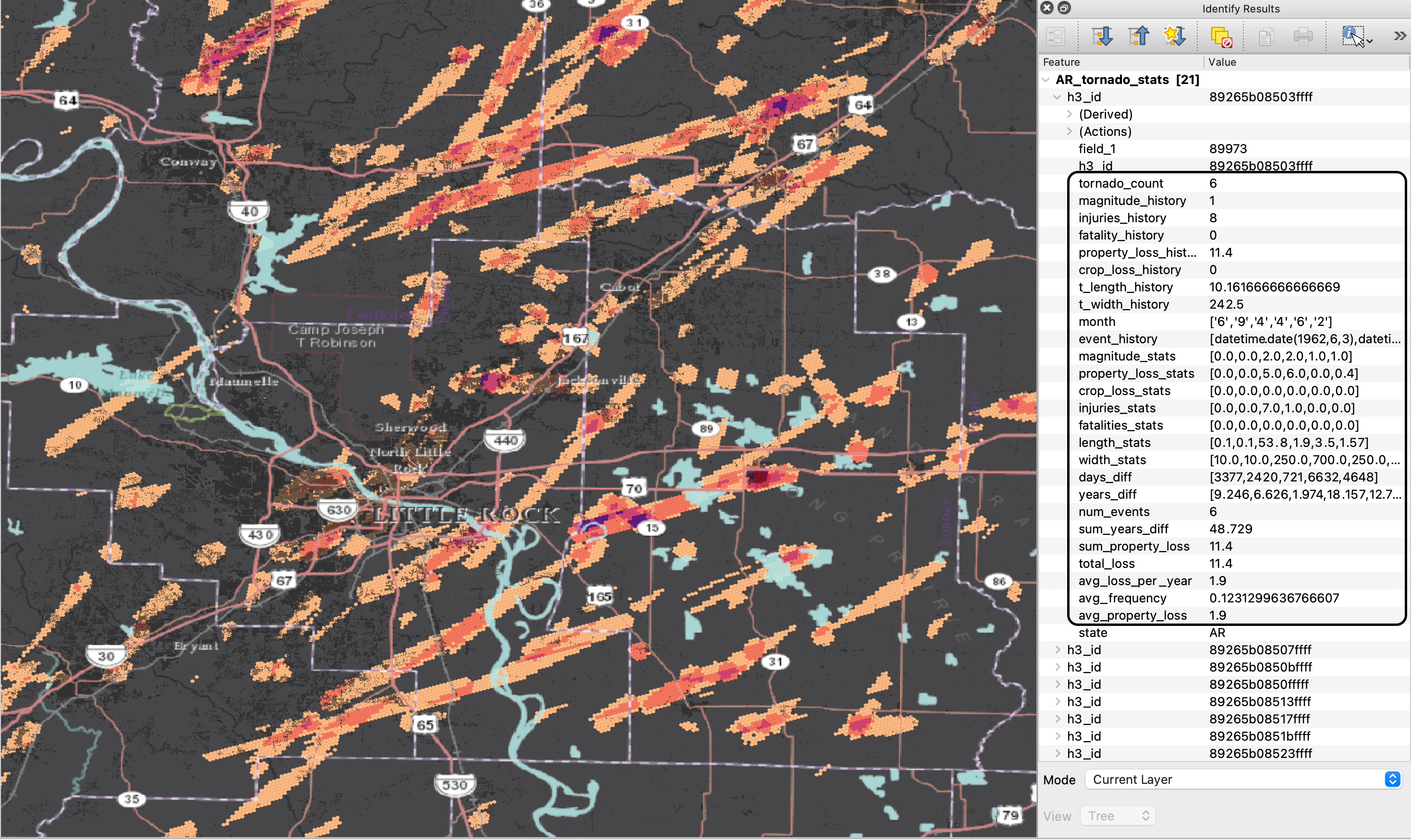
Tornado Statistics for Underwriting

annual_probabilities is a measure of how often tornado events occur in a particular hexagon, on average.

• It is calculated by dividing the total number of tornado events in a hexagon by the sum of the years difference between each event.
• This measure is computed by dividing the total number of tornado events in a hexagon by the sum of the time differences between each event.
• For instance, if a hexagon experienced 5 tornado events with time differences of 1, 2, 3, 4, and 5 years, respectively, the sum of the time differences would be 15.
• Consequently, the average frequency of tornado events in this hexagon would be 5/15 or 0.33 events per year on average.

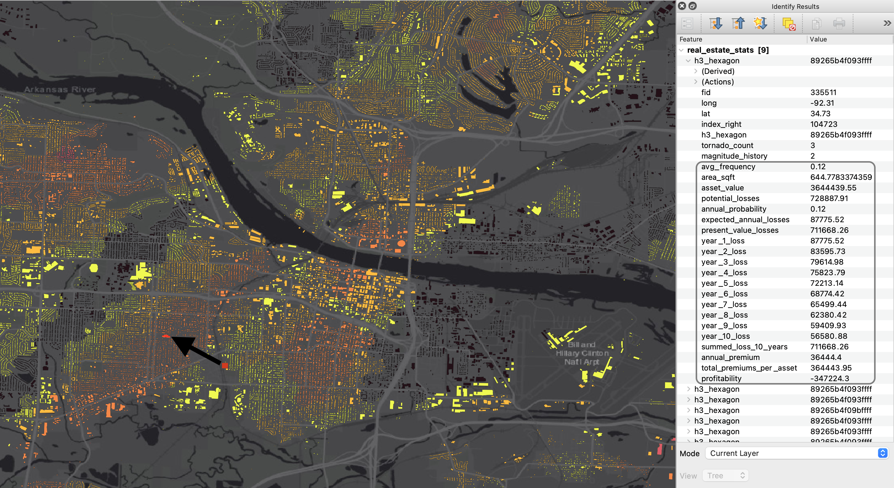
Expected Loss

In the insurance industry, the Annual Expected Loss (AEL) equation is a statistical tool used to estimate the amount of money an insurer is likely to pay out in claims over a year. It is calculated by multiplying the Probability of Loss (PoL) by the Expected Loss Amount (ELA).

Mathematically, the equation for Annual Expected Loss is:

• AEL = PoL x ELA

where:

• PoL is the probability of a loss occurring within a given period of time (usually one year)
• ELA is the expected loss amount for a single loss event To calculate the Annual Expected Loss, an insurer will typically use historical data to estimate the PoL and ELA for a particular type of insurance policy (Rejda & McNamara, 2021).
• The insurer may also factor in other variables, such as the level of risk associated with a particular policy, to refine their estimate of the AEL. By estimating the AEL, insurers can better understand the potential financial impact of insuring a particular risk and set appropriate premium rates to cover their expected losses (Rejda & McNamara, 2021).

Other calculations to be made…

• Value at Risk (VaR)

import numpy as np

# Assuming a normal distribution, we will use the scipy library for VaR calculation
from scipy.stats import norm

# Confidence level (e.g., 95%)
confidence_level = 0.95

# Calculate portfolio loss distribution (sum of expected losses)
portfolio_loss_distribution = df['expected_loss'].sum()

# Calculate standard deviation of the portfolio loss distribution
# You can use historical data or other methods to estimate the standard deviation
portfolio_loss_std_dev = np.std(df['expected_loss'])

# Calculate VaR at the specified confidence level
VaR = norm.ppf(confidence_level, loc=portfolio_loss_distribution, scale=portfolio_loss_std_dev)

print("Value at Risk (VaR):", VaR)

• Tail Value at Risk (TVaR)

# Calculate TVaR at the specified confidence level
# First, we need to find the probability density function (PDF) value at VaR
pdf_at_VaR = norm.pdf(VaR, loc=portfolio_loss_distribution, scale=portfolio_loss_std_dev)

# Then, we calculate the tail probability beyond VaR (1 - confidence level)
tail_probability = 1 - confidence_level

# Finally, we calculate the TVaR using the formula: VaR + (pdf_at_VaR / tail_probability)
TVaR = VaR + (pdf_at_VaR / tail_probability)

print("Tail Value at Risk (TVaR):", TVaR)

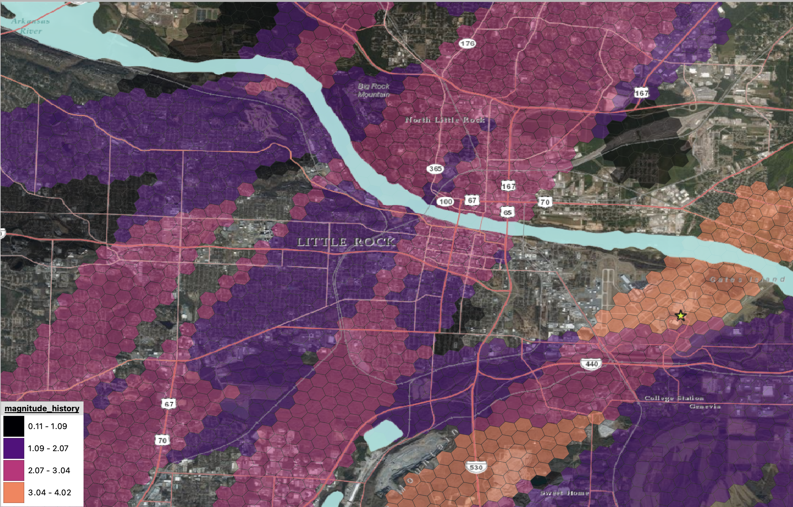
Tornado Risk of Arkansas Real Estate properties

• The map above shows real estate properties that have encountered at least 1 tornado (up to 7) in a 90-year period.

• Black symbols show real estate that has not encountered an tornado.

• In the accompanying map, we illustrate real estate properties that have encountered at least one tornado (up to seven) within a 90-year period.
• The properties that have not encountered any tornadoes are represented by black symbols.
• The map also highlights the real estate properties most at risk, displayed in yellow.
• It is important to note that real estate located in areas prone to tornadoes is more likely to incur losses.

• we look up each property and return a precise tornado probability score
• annual_probability has a geographic precision of 110m^2
• basis for the expected_annual_loss equation

Reference:

Rejda, G. E., & McNamara, M. J. (2021). Principles of Risk Management and Insurance (14th ed.). Pearson.